Identifying network-throughput bottlenecks with trace recording

I recently launched an investigation in order to identify bottlenecks in Genode’s network packet throughput. This endeavour sparked off a new tool, the trace recorder, for recording component traces in Genode that I want to present to you in this article.

Identifying bottlenecks in network throughput can be particularly challenging as there are a lot of variables that may affect the result. Particularly on Genode, network packets traverse multiple components between the actual application and the network controller. We must therefore often look into quite complex scenarios (like Sculpt) instead of debugging components in isolation.

The GENODE_LOG_TSC macros (see Performance analysis made easy), are a simple, yet powerful, profiling tool when it comes to single components. For my investigation, however, I needed something that shows how multiple components interact. A few years ago, I had a joyful experience using the Linux Tracing Toolkit next generation (LTTng), thus I wanted to bring something similar to Genode using its lightweight event-tracing infrastructure. The result is the trace-recorder component that is released with 22.08.

Before explaining the details of the trace recorder though, let’s start with the background story that illustrates the employment of this new tool.

Background story

The very origin of this was about a year ago when I noticed that the native Falkon browser achieves rather low download rates on Sculpt (#4203). Back in December, Norman suggested having a look at the packet fill states since he suspected that eager signalling of the packet-stream interface could lead to frequent back-and-forth switching between components instead of batching. This idea hibernated for a while. This summer, I have eventually written a test component called "nic_perf" to first benchmark the packet-stream interface in isolation and then add more components such as the NIC driver and NIC router. The nic_perf component simply sends and/or receives a stream of UDP packets and periodically outputs the throughput.

In order to get a baseline, I benchmarked the throughput of the packet-stream interface with two nic_perf components: One component transmitting a stream of UDP packets and the other receiving the same, without any packet inspection or copying. In this scenario, I achieved 13000Mbit/s on a Thinkpad T490s (with i7-8565U CPU), 9000Mbit/s on an Thinkpad X260 (with i5-6200U CPU), and 1300Mbit/s on a Cortex-A9 @ 666MHz. Adding the NIC router in between the two nic_perf components, however, dropped the throughput down to approx. 10% of the above results. Luckily, I had already drafted the trace-recorder component and could have a look at the signalling between the involved components and the fill states of the submit and ack queues with the TraceCompass tool.

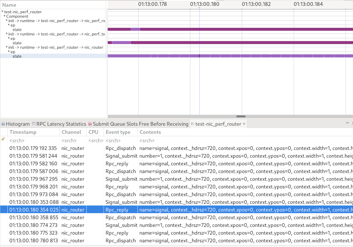
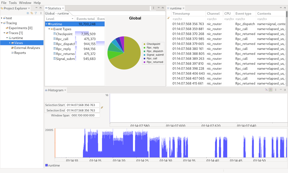
TraceCompass visualisation

The above figure shows a TraceCompass screenshot with a Gantt-like chart and a textual representation of the trace. The light purple colour indicates thread activities whereas the dark purple colour shows that a thread is waiting. We can see that the NIC router signals itself multiple times and is not interrupted by nic_perf_rx or nic_perf_tx. More precisely, it processes batches of 32 packets (following its default "max_packets_per_signal" config option), hence eager signalling was not a problem (at least on base-nova). Yet, the NIC router consumed most of the CPU time.

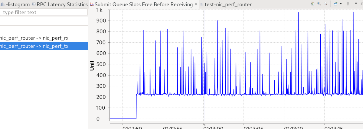
In the process, I also instrumented the nic_perf component and implemented a custom analysis for TraceCompass to visualise the fill states of the packet-stream queues. The screenshot below depicts how many slots (of the 1023) are free in the submit queue when nic_perf_rx is signalled. It clearly shows that the submit queue is never full nor empty, which is exactly what we want to see.

Visualisation of the submit queue fill state

To narrow down where the NIC router spends its time, I instrumented the router using GENODE_LOG_TSC. First, I was a bit baffled seeing that neither memcpy nor the checksum calculation was contributing significantly to the processing time of a packet. Instead, it turned out that most of the time is spent exception handling (i.e. between throw and catch) when it tried to find the correct routing rule. Martin thankfully provided a fix that immediately tripled the throughput.

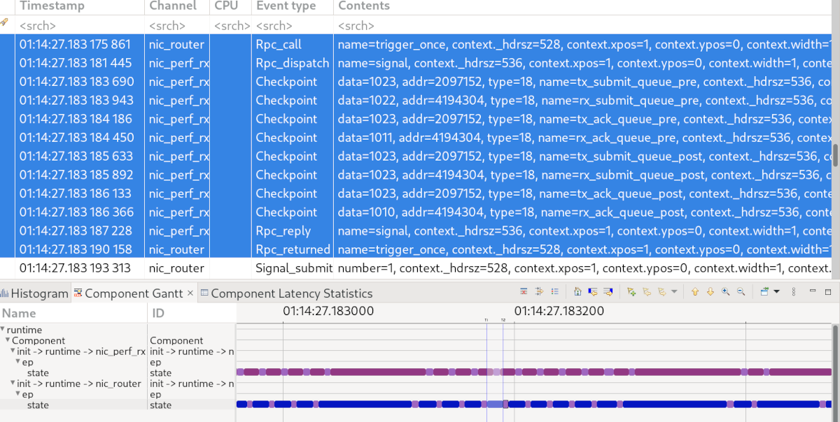
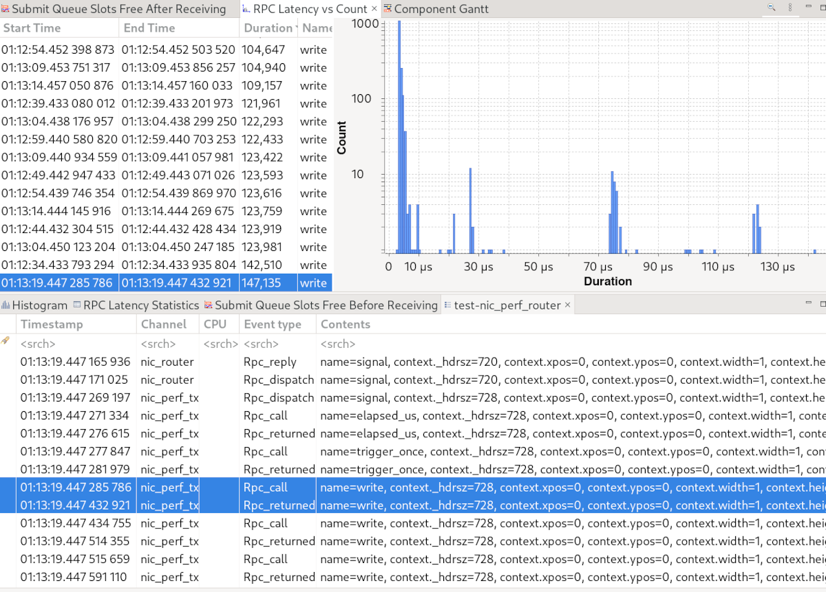
Up to this point, I used an IP routing rule. When I switched to a UDP rule, however, I observed another slow down that required further investigation. Instead of digging into the (unfamiliar) code of the NIC router, I recorded some traces. As shown in the screenshot below, the traces uncovered that the router issued a trigger_once RPC (blue colour) for almost every packet. A glance into the code explained this situation: Since the NIC router caches the active routes, it maintains a timeout to remove a route from the cache once it became inactive. It therefore updated the timeout for every packet and since the new deadline moved a tiny bit into the future, the timeout framework issued a trigger_once RPC. In a joint effort, we persuaded the NIC router to be less accurate with these timeouts.

Most of the NIC router’s time is spent in trigger_once RPCs

Along the way, we identified the following (minor) tweaks that contribute to the overall speedup of the NIC router:

• On base-hw, eager signalling thwarted our previous optimisations. By only emitting packet-stream signals once the NIC router processed all available (or up to max_packets_per_signal) packets, we enforce batch processing of packets.

• Since the batch size is controlled by the max_packets_per_signal attribute, we increased the default value from 32 to 150 as this brought significant throughput benefits.

• We implemented incremental checksum updates according to RFC1071 to avoid complete checksum recalculation when forwarding UDP/TCP packets.

As a result, we boosted the NIC router’s UDP throughput up to approx. 45-55% of the initial baseline (depending on the hardware). Given the complexity of the NIC router, and the involved routing and copying, I consider this is a decent performance.

Next, let’s dive into the details of the trace-recorder component that took a substantial part in these optimisation efforts.

Trace-recorder component

Inspired by LTTng and Wireshark, the trace recorder is able to record event traces as well as packet traces.

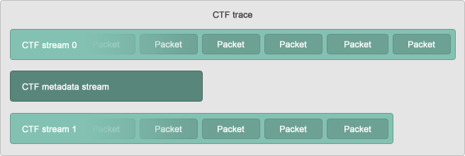
With respect to event traces, I came across the Common Trace Format when using LTTng. A CTF file is hierarchically structured into event streams that are made up of one or multiple packets. A packet bundles one or multiple binary events that occurred in a certain time frame. The format of each stream’s events is specified in the trace’s metadata, which uses the Trace Stream Description Language.

Structure of a CTF trace. (Source: https://diamon.org/ctf/)

CTF perfectly fits the job because it is compact and scales pretty well due to its hierarchical structure. Another cool thing about CTF is that there are tools available for analysis, namely babeltrace and TraceCompass.

For packet tracing, on the other hand, I chose pcapng simply because Wireshark can read it.

Design

Let’s first recapitulate what facilities Genode already provides.

At the very basis resides the TRACE service that is implemented by core. It enables a monitor component (the TRACE client) to control whether and how the running components are traced. For this purpose, it provides policy modules (containing code) and a trace buffer for every traced thread. The policy code is called by the traced thread whenever a trace point is passed. When called, the code returns the data to be captured in the trace buffer. Trace points have been defined to capture component interactions (RPC dispatch, RPC reply, RPC call, RPC returned, signal submit and signal receive).

So far, the event tracing has been used for capturing textual representations of events. With the trace logger and the VFS plugin there are two corresponding monitor components. The trace logger periodically writes the trace-buffer content to the LOG session whereas the VFS plugin provides access to a trace buffer via a File_system session. In addition to the aforementioned trace points, components can be instrumented using the Genode::trace() function that is similar to Genode::log() but calls the trace policy instead of using a LOG session. Since verbose LOG output can impede the timing and/or performance of a component, redirection of LOG output to the trace buffer is another option.

Along with the event tracing, the TRACE service also provides access to a thread’s execution time. This is used by the CPU-load display and the log-based top component.

The trace recorder fits into this tool kit as another monitor component that also supports binary trace data. Instead of logging the trace-buffer content, it writes the trace data into a target file system. For every trace session, the trace recorder creates a new sub-directory named by the current date and time taken from an Rtc session.

The trace recorder consumes the trace events from the trace buffer at (configurable) periodic intervals and forwards them to the corresponding writer backend (currently CTF or pcapng) depending on the event type. For this purpose, the data returned by the trace policy must be of type Trace_recorder::Trace_event, which is a template that adds a type field at the very beginning of each trace-buffer entry (currently distinguishes between CTF and pcapng).

CTF tracing

 GENODE_TRACE_CHECKPOINT(data);
 GENODE_TRACE_CHECKPOINT_NAMED(data, "name");

 GENODE_TRACE_DURATION(data);
 GENODE_TRACE_DURATION_NAMED(data, "name");

Packet capture (pcapng)

For packet capture, I added a trace_eth_packet() method to the trace policy API, which takes an interface name, a direction, a pointer to the packet data, and the packet size as arguments. Similar to the CTF tracing, the file gems/include/trace_recordcer/pcapng.h contains the declaration of the pcapng-formatted events so that the pcapng writer of the trace recorder only needs to apply little modifications before writing the data to the file system in a .pcapng file. The pcapng writer uses the component’s label as file name and path. The trace of init -> runtime -> nic_router would therefore land in a <date+time>/init/runtime/nic_router.pcapng file.

Currently, the trace_eth_packet() trace point is only used by the NIC router and must be enabled separately via its trace_packets attribute (see NIC router README). You can create a corresponding trace point (e.g. in a NIC driver) using Genode::Trace::Ethernet_packet from base/trace/events.h.

For every trace-recorder period, a new section is written to the pcapng file. A section contains the packet data from all interfaces. Although this is supported by the pcapng specification, I noticed that Wireshark has not always displayed the interface names correctly. The interfaces are assigned unique identifiers (incrementing unsigned 32-bit number) within each section in order to be referenced by the traced packets. Depending on the order of appearance, the same interface may get varying identifiers in different sections. However, Wireshark appeared to ignore this fact. Nevertheless, I was able to work around this issue by filtering on IPs instead of interface names.

Configuration

The configuration of the trace-recorder component is fully documented in its README.

As already mentioned, the trace recorder requires write access to a File_system and to an Rtc service. A ready-to-deploy package for Sculpt 22.10 is available in my depot. Further examples are found in the run scripts gems/run/trace_recorder*.run.

For now, let’s have a look at an example to illustrate how the trace recorder is configured:

 <config period_ms="5000" target_root="/" enable="yes">
     <vfs> <fs/> </vfs>
     <policy label_suffix="dynamic_rom" policy="ctf0">
        <ctf/>
     </policy>
     <policy label_suffix="nic_router1" thread="ep" policy="pcapng">
        <pcapng/>
     </policy>
     <policy label_suffix="nic_router2" policy="ctf0_pcapng">
        <ctf/>
        <pcapng/>
     </policy>
  </config>

The config takes attributes for the sampling period of the trace buffers and the root directory for writing the trace data. Moreover, it has an enable attribute. Whenever the trace recorder changes state from disabled to enabled, it goes through the list of trace subjects and looks for a matching policy following the established label-based matching in combination with the thread attribute. When a matching policy was found, the policy module specified by the policy attribute is inserted and a trace buffer will be attached. The buffer size can be controlled by the buffer attribute. Currently, there are three policy modules available: ctf0 for CTF tracing, pcapng for packet capture, and ctf0_pcapng for simultaneous CTF tracing and packet capture. Note that the packet capture length is limited to 100 bytes to reduce buffer and file sizes.

Each policy node also takes a list of writer backends that shall be activated for each matching subject. Currently, there is a <ctf/> backend consuming the CTF trace events and a <pcapng/> backend consuming the pcapng trace events.

Analysis of CTF traces

After recording a CTF trace, we are able to conduct analyses with the collected data. Babeltrace is the reference parser implementation of CTF. It comes with a C API and Python 3 bindings. TraceCompass is an Eclipse-based tool for visualisation and analysis of CTF and other trace formats. I particularly like the interactive navigation through a trace and across different views. In this section, I am going to provide a brief introduction in how to use TraceCompass with CTF traces from Genode.

In order to feed the CTF output from the trace recorder into TraceCompass (or babeltrace), we must serve it on a single plate. In other words, TraceCompass expects all trace files to reside in one directory. Since the trace recorder writes the files into different directories following the hierarchical system structure, I manually copy (and rename) each thread’s trace file into a new directory and garnish it with one of the metadata files (they are all identical). Note that TraceCompass uses the directory name as the name of the trace and the file names as channel names.

After opening TraceCompass (requires at least version 7.3), select File -> Open Trace and select any of the trace files. TraceCompass automatically imports all CTF files in the same directory and presents you with a list of trace events. Via Window -> Show View, you can also add a histogram or statistics view.

TraceCompass with histogram and statistics

These views are nice to look at but do not provide much insight in our case, yet we can define our own analysis in an XML file (see Data driven analysis). With this, one is able to define how the trace events modify TraceCompass’ internal state system. Based on this, a Gantt-like time graph view (as shown in the beginning) or an XY chart (used for the "Submit Queue Slots Free Before Receiving" view) can be defined. Moreover, one can specify state machines to detect certain patterns and measure latencies. A set of views is automatically generated for the latter.

Another, more powerful, way is to write an EASE script. Yet, I took the XML road and implemented a component-interaction analysis and a checkpoint analysis. The component-analysis XML provides a time graph view for a thread’s state, i.e. whether it is ready, waiting for an RPC, etc. that you have already seen in the beginning. It also defines an RPC latency analysis and an analysis for the duration of thread activities. The latter is not exact but turned out to be quite useful in identifying long-running activities. The screenshot below shows the "RPC Latency vs Count" view provided by the RPC latency analysis.

TraceCompass’ "RPC Latency vs Count" view

The checkpoint-analysis XML provides a latency analysis of code sections instrumented with GENODE_TRACE_DURATION or GENODE_TRACE_DURATION_NAMED macros.

In order to import an XML analysis, right click on Traces in the project explorer and select Manage XML analyses.

Powers and limitations

I’d like to emphasise that the trace recorder is not a silver bullet but only one tool in the kit. Other useful tools are the GENODE_LOG_TSC and GENODE_TRACE_TSC macros as well as the trace-logger component. Let me therefore clarify the pros and cons of the trace recorder so that you become able to choose the right tool for every task.

The trace recorder plays its tricks as soon as multiple components (or threads) are involved. Typical traced events are component interactions (RPCs and signals). By recording every event with a timestamp, we are able to analyse latencies, calculate statistics, or have a look at certain event sequences we are interested in (e.g. using custom TraceCompass analyses). Furthermore, as it is designed to work with binary trace data, it becomes useful when a lot of trace events must be captured that would require too much memory in textual representation. The downside is that the trace recorder may still generate a lot of data depending on the event frequency.

Moreover, you should be aware of the fact that it uses Trace::timestamp(), which maps to the CPU’s cycle counter. On older x86 CPUs, the cycle counter was not constant but depended on the current frequency. On ARM CPUs, the cycle counter stops once the CPU is set to idle mode by the wfi instruction.

Please note that the trace recorder only goes through the trace subjects once (when enabled) to insert a policy module and attach a trace buffer in order to save computational resources for processing large amount of trace-buffer data. In consequence, any subject that does not exist when the trace recorder gets enabled, will not be traced.

References

Github issues:

• #4555: NIC router optimisations

• #4536: Eliminate exceptions in NIC router

• #4352: Trace recorder

• #4203: Bad throughput for native Falkon browser

3rd-party tools and documentation:

• CTF spec

• pcapng

• LTTng

• babeltrace

• TraceCompass

• TraceCompass’ Data driven analysis

Release notes:

• Release Notes 13.08: Light-weight event tracing

• Release Notes 15.08: CPU-load display

• Release Notes 17.05: Log-based CPU-load display

• Release Notes 18.02: trace logger

• Release Notes 19.08: VFS trace plugin

• Release Notes 20.05: redirection of LOG output to TRACE events

READMEs and documentation:

• Genodians article: Performance analysis made easy

• NIC router README

• Trace recorder README

Trace recorder resources:

• componentanalysis.xml

• checkpoint.xml

• metadata